You are viewing an older revision! See the latest version
PID
A proportional-integral-derivative controller (PID controller) is a generic loop feedback mechanism. It measures a process variable (e.g. temperature), and checks it against a desired set point (e.g. 100 degrees celsius); it then attempts to adjust the process variable by changing a controller output (e.g. PWM signal to an electric heater) which will bring the process variable closer to the desired set point.
The wikipedia article on PID controllers is an excellent place to start in understanding the basic concepts. The controlguru website also contains a wealth of easy to digest information on how to implement and tune a PID controller.
As these resources can already explain the fundamentals and implementation of a PID controller, this page will detail the PID library and then present an example of putting it into practice.
Software
The PID software runs a loop at a set interval, and performs the following calculation:

Where
- CO is the controller output
- CObias is an optional, user set bias for the controller output
- Kc is a proportional tuning constant
- e(t) is the error at time t
- Ti is an integral tuning constant
- Td is a derivative tuning constant
- PV is the process variable
- dt is the rate the loop runs at
The controller works in percentages during the calculations and then scales relevant outputs back into real world values.
Initialization
When a PID object is created, the three tuning constants (Kc, Ti, Td) and an interval time are passed as parameters. By default the controller starts in manual mode - whenever the controller is changed to auto mode, the working variables are reset (according to the current limits) which allows for "bumpless" transfer between manual and auto mode. The input and output limits are set as 0.0-3.3 [volts], and the tuning constants are slightly modified to make things easier during calculations. Finally, appropriate variables (such as the controller output and process variable) are initialized to zero before the main loop method is attached to a Ticker which runs at the rate passed in by the user.
Application
In order to set up a PID object for use in a specific application, a typical initialization and loop might look like this.
[Not found]
Example: Velocity Control
This example will show how to use the PID controller library and a brushed DC motor with a quadrature encoder and H-bridge to perform velocity control.
We can calculate the velocity of the motor by taking two samples of the quadrature encoder's pulse count in a short interval and then dividing the difference between them by the length of the interval to get the number of pulses per second.
We could turn pulses per second into a more familiar unit, such as metres per second, but we want to try and choose a process variable which is as closely related to what we're measuring as possible; and since what we're measuring (pulses per second) is directly proportional to the velocity, it should provide a much better value to work with during our PID calculations.
Our process variable will therefore be the number pulses per second we've read, and our controller output will be the PWM signal's duty cycle to the H-bridge.
Tuning Method
There are many ways to tune the constants in a PID controller, including simple trial and error; the method presented on controlguru involves fitting a simple first order plus dead time (FOPDT) dynamic model to process test data that we take - a lot easier than it sounds! This is the method we will follow, but it is not the only way.
Step Test
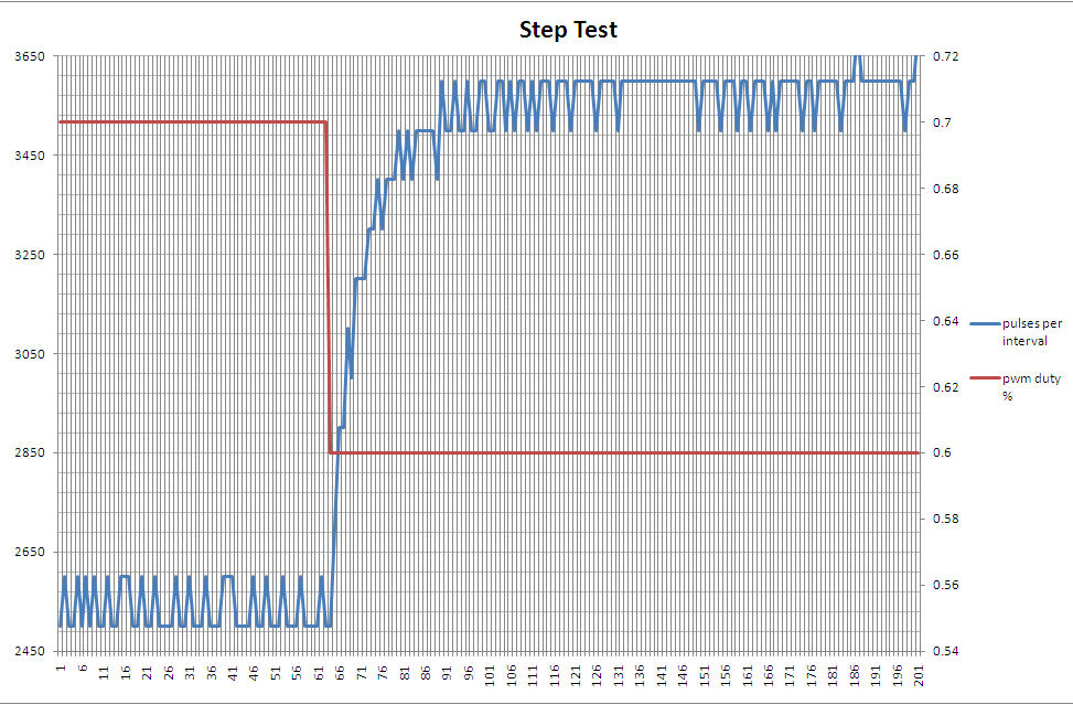
The first we need to do, is observe how our process variable changes with respect to controller output. We'll do this by performing a step test - after setting our controller output to a specific value and observing our process variable, we will then "step" our controller output to a new value and watch what happens to our process variable.
Here are the results.

The number of counts per second were observed while the PWM duty cycle was 70%, and after it was stepped to 60%.
Process Gain Constant
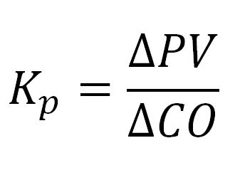
The process gain constant or Kp describes how the process variable changes when the controller output changes. It is calculated in the following way:

We can use the data from our step test to calculate to Kp.

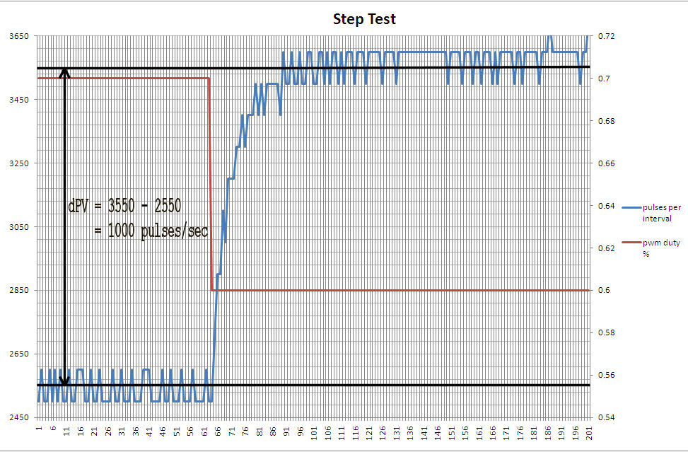
dPV = 1000, and dCO = -0.1; when talking about the controller output, we will use how far "on" or "off" it is as a percentage in our calculations to make things easier. Therefore dCO = -10%.
Kp = dPV / dCO = 1000 / -10% = -100 counts per second/%
Process Time Constant
The process time constant or Tp describes how fast the process variable changes when the controller output changes. It is calculated by measuring the time it takes from when the process variable first begins to respond to a step in the controller output, to 63% of the total change in the process variable from a step in the controller output. The 63% comes from solving the FODPT differential equation and is beyond the scope of this page.
Our dPV = 1000, so 63% would be when our process variable has increased 630 counts.

Since the ticks on the x-axis are 0.01s intervals we obtain:
Tp = 72 - 64 = 8 = 0.08s
Dead Time Constant
The dead time constant or [theta]p describes the delay between a change in the controller output and when the process variable first starts to respond.

On our graph it appears the change is almost instantaneous - we should bear in mind that it's impossible for the dead time to be less than the sample time (in our case 0.01s), and also it's generally better to be conservative with the value.
From the graph:
[theta]p = 64 - 63 = 1 = 0.01s
Constants
We have now estimated the constants required for our controller; they are:
| Kp (Process Gain) | -100 counts per sec/% |
| Tp (Process Time) | 0.08s |
| [theta]p (Dead Time) | 0.01s |
Proportional Controller
A proportional or P-Only controller has no integral or derivative action. A moderate controller gain, or Kc, can be calculated for a P-Only controller in the following way (see controlguru for details):

Giving Kc = -0.025... %/counts per second
We should be careful not to read too much into these constants; an increase in decimal places will probably not relate to an increase in performance.
Before we plug this into our controller, we have to change Kc into a dimensionless constant as the PID library works in the percentage domain.

The minimum value for our process variable is 0 (when the motor is stationary), and it achieves approximately 10500 counts per second when run at full speed. Therefore we get:
Kc = -0.025 * (10500/100) = -0.025 * 105 = -2.6
We'll use the following code to test our controller.
#include "PID.h"
#include "QEI.h"

#define RATE 0.01
#define Kc   -2.6

PwmOut motor(p23);
DigitalOut brake(p19);
DigitalOut direction(p28);
QEI qei(p29, p30, NC, 624);
PID controller(Kc, 0.0, 0.0, RATE);

Timer timer;

LocalFileSystem local("local");

//Working variables.
int pulses     = 0;
int prevPulses = 0;
//Controller output.
float pwmDuty  = 1.0;
float setPoint = 3000;
//Process variable.
float velocity = 0.0;

int main() {


    motor.period_us(50);
    motor = 1.0;
    brake = 0.0;
    direction = 0;
    motor = pwmDuty;

    controller.setInputLimits(0.0, 10500);
    controller.setOutputLimits(0.0, 1.0);
    //PWM duty = 0.0 => motor completely on.
    //PWM duty = 1.0 => motor completely off.
    controller.setBias(1.0);
    controller.setMode(AUTO_MODE);

    FILE* fp = fopen("/local/steptest.csv", "w");

    controller.setSetPoint(setPoint);
    timer.start();

    while (timer.read() < 3.0) {

        pulses = qei.getPulses();
        velocity = (pulses - prevPulses) / RATE;
        prevPulses = pulses;
        controller.setProcessValue(velocity);
        pwmDuty = controller.getRealOutput();
        motor = pwmDuty;
        fprintf(fp, "%f,%f\n", velocity, setPoint);
        wait(RATE);

    }

    motor = 1.0;

    fclose(fp);

}
The graph below shows our results.

As seen, our P-Only controller is experiencing "offset"; that is, the set point it reaches is offset from the actual set point we want it to reach. This problem can be solved by using a PI controller which introduces an integral term that updates the output based on the sum of the previous errors.
As we increase the proportional constant, the offset is reduced but at the cost of overshoot (going further than our set point before dropping down to the right value) and also increasingly wild oscillations. A proportional constant four times the size of a moderate value will give results that look like this:

PI Controller
We'll use the same constants we calculated before to work out two tuning parameters; the first will be the one we met before in the P-Only controller, that is the controller gain Kc, and the second will be the reset time Ti.
For the PI controller:
![]()
Where
- Kp = Process gain, calculated earlier from step test
- Tp = Process time, calculated earlier from step test
- [theta]p = Dead time, calculated earlier from step test
- Tc (moderate) = max(1 * Tp, 8 * [theta]p)
- Reset time Ti = Tp
This gives us the following values for the tuning constants:
- Tc = max(0.08, 0.08) = 0.08
- Kc = (1 / -100) * (0.08 / (0.01 + 0.08)) = -0.009
- Kc (dimensionless) = -0.009 * (10500/100) = -0.9
- Ti = 0.08
Plugging these into our controller gives the following results:

Not bad at all! No overshoot, and only a little delay in reach the set point which it stays at comfortably.
Let's see what happens if we choose more conservative, or aggressive tuning parameters. Ti will remain equal to Tp but we'll use the following values for Kc.
- Aggressive tuning
- Tc = max(0.1 * Tp, 0.8 * [theta]p) = max(0.008, 0.008) = 0.008
- Kc = (1 / -100) * (0.08 / (0.01 + 0.008)) = -0.04
- Kc (dimensionless) = -0.04 * (10500/100) = -4.7
- Conservative tuning
- Tc = max(10 * Tp, 80 * [theta]p) = max(0.8, 0.8) = 0.8
- Kc = (1 / -100) * (0.08 / (0.01 + 0.8)) = -0.001
- Kc (dimensionless) = -0.001 * (10500/100) = -0.105

While the aggressive tuning has a faster response, we also see a big overshoot and lots of oscillation which takes a long time to settle. The conservative tuning doesn't overshoot but takes a lot longer to get closer to the set point.
The moderate tuning gives adequate performance and was tested on a range of changing set points.
![]()
With just a little overhead, we've managed to select very favourable tuning constants for our PID controller. Even better values could be selected with the appropriate software, but this example has shown you can do it by eye on simple graphs.
Adding the derivative component
For most applications, a PI controller might be sufficient for control, as shown in this example.
Adding the derivative component to the controller is much like adding the integral component; there is simply an extra tuning constant to calculate from our original three values for Kp, Tp, and [theta]p.
More information including some common pitfalls when adding the derivative can be found on the controlguru website.
Library
[Not found]