Drawing Robot (with drawing software)
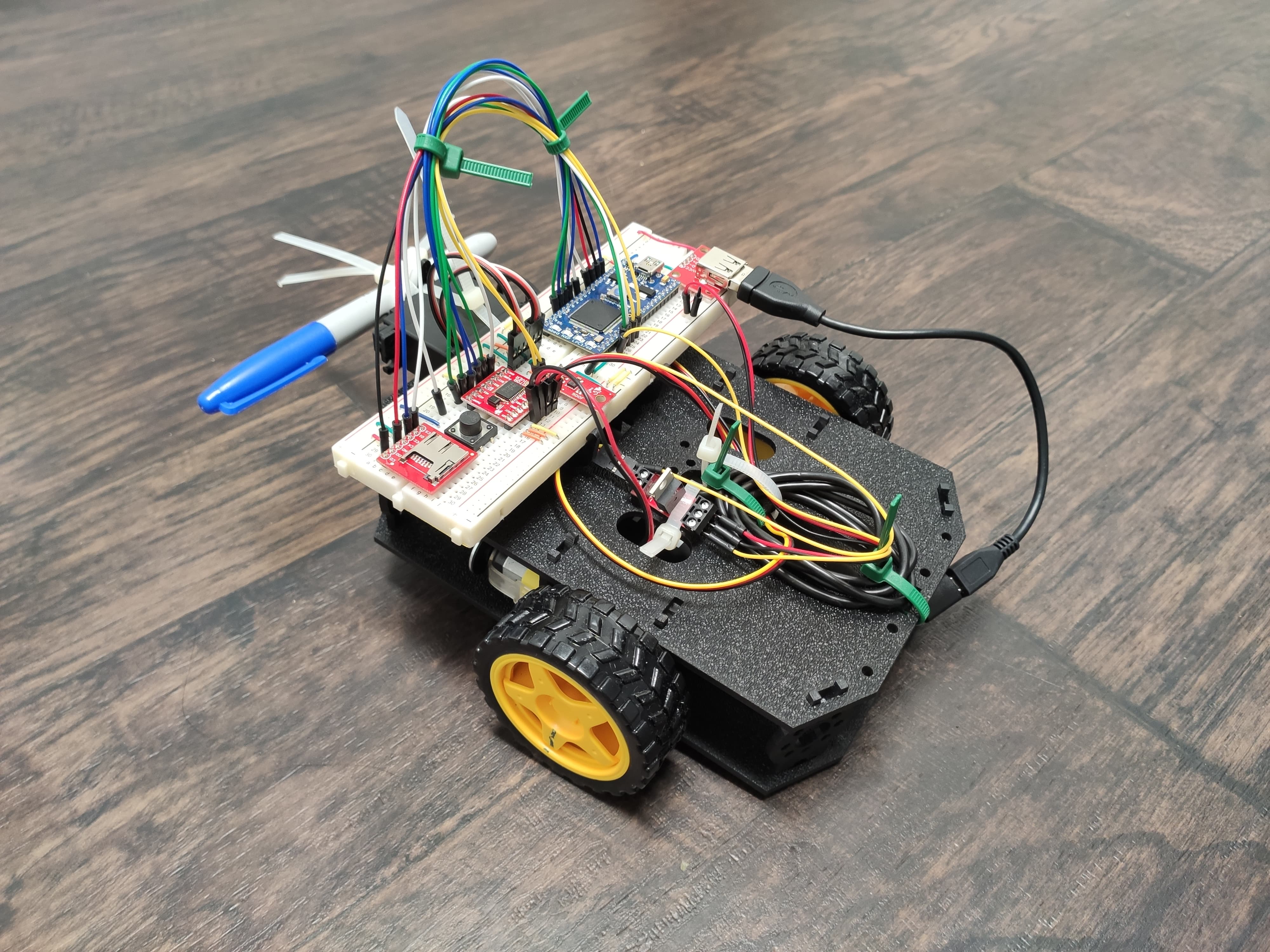
Team members
- Arnaud Billon
- Alexandre Mazgaj
Goals
Our base idea in this project was to tackle the issue of autonomous robotics using our robot kit:
- Design a robot able to autonomously replicate a drawing on paper lying on the floor, by operating a pen on and off the surface.
- The drawing would be created and uploaded using dedicated desktop software, possibly in a wireless manner.
- The framework should also provide minimal calibration and debugging capabilities.
Achieved Design Description
Given the difficulty of the task at hand and the differents setback we encountered, we had to reconsider our solution:
- We designed a simple Python GUI, in which it is possible to create a drawing in the form of disconnected paths , the user decides of the shape, number of nodes and Pen actuation timings.
- The drawing can be exported to a csv format and uploaded using a SDcard.
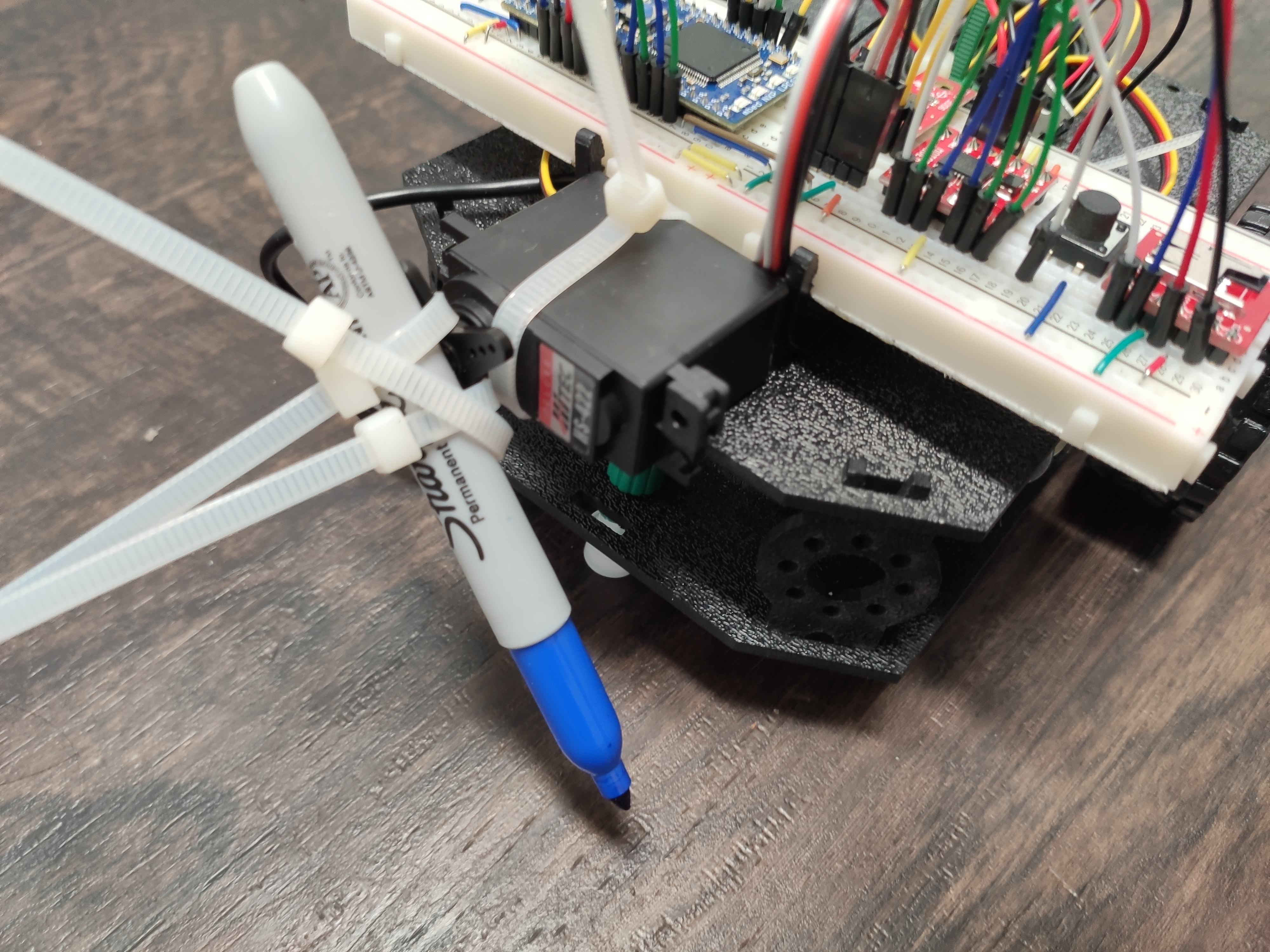
- The robot tries to autonomously reproduces the pattern, by operating a Pen tied to a Servo Motor.
Despite different approaches to the problem, we did not reach significant accuracy to reproduce complex design, namely we struggled with the measurement of the robot global angle. However we identified the point that needs to be worked on to get such system working efficiently.
Commented Slideshow
The slideshow summarizes our work and the things presented on this page, it has embeded recorded commentaries. It is available at this URL:
The recorded audio commentaries are triggered automatically, but can be restarted again using the "Sound" button in the lower right corner.
Components
Parts list
- 1x mbed LPC1768 (https://www.sparkfun.com/products/9564)
- 1x Shadow bot chassis (https://www.sparkfun.com/products/13301)
- 2x Wheels (https://www.sparkfun.com/products/13259)
- 2x DC Motors (https://www.sparkfun.com/products/13302)
- 1x H-Bridge (https://www.sparkfun.com/products/14450)
- 2x Hall effect encoders (https://www.sparkfun.com/products/12629)
- 1x Servo motor (https://www.sparkfun.com/products/11965)
- 1x MOSFET (https://www.sparkfun.com/products/12959)
- 1x microSD card (https://www.sparkfun.com/products/14832)
- 1x microSD card reader (https://www.sparkfun.com/products/544)
- 1x Pushbutton (https://www.sparkfun.com/products/9190)
- 1x portable battery
- 1x USB Type A Female connector (https://www.sparkfun.com/products/12700)
- 1x Plastic Caster (Unknown origin)
- 1x Sharpie (https://www.sharpie.com/all-markers/specialty/extreme/SHExtremeBlackFine)
- Handful of zipties for keeping parts in place and cable management
Wiring
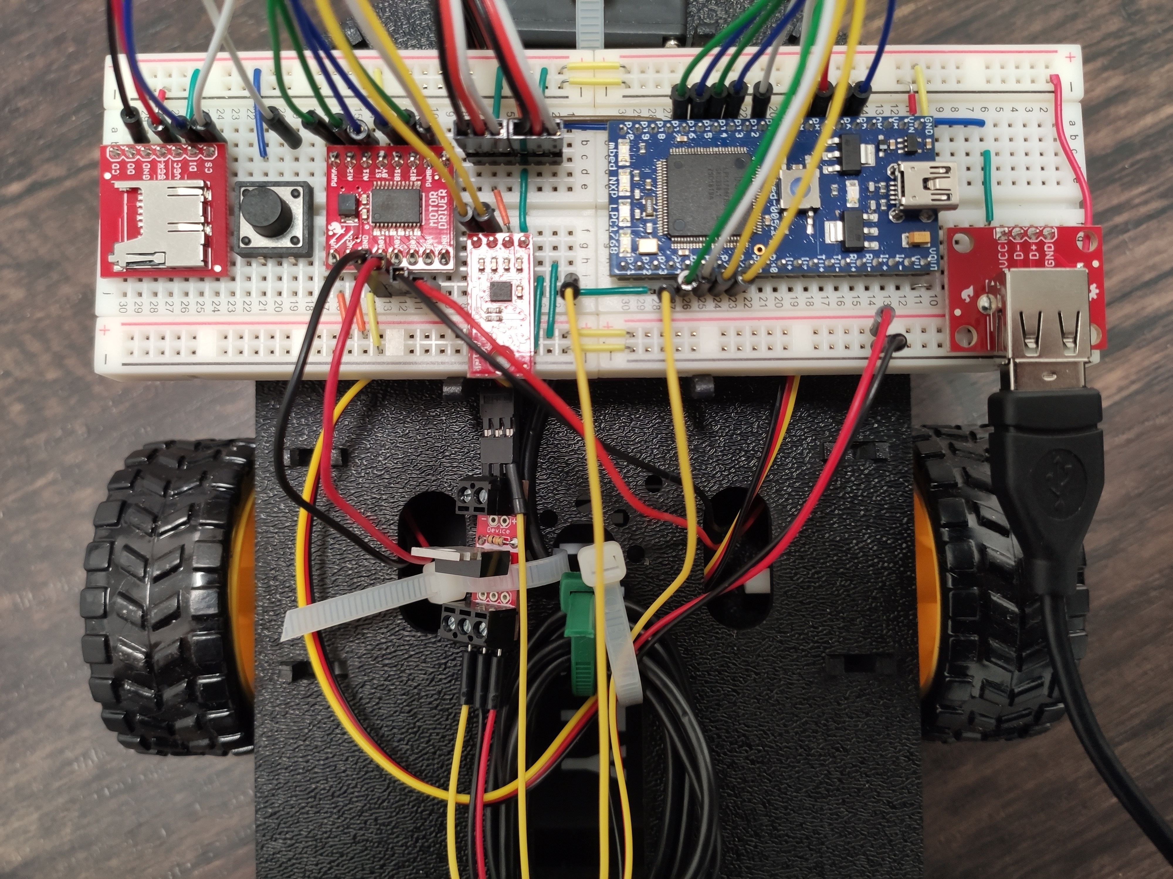
H-bridge and DC motors
The H-bridge controls the two DC motors connected to the wheels.
| MBED | H-bridge | Left DC motor | Right DC motor | External DC supply |
|---|---|---|---|---|
| VCC | VOUT | |||
| VCC | STBY | |||
| VM | 5V | |||
| GND | GND | GND | ||
| p13 | AI1 | |||
| p14 | AI2 | |||
| p15 | BI1 | |||
| p16 | BI2 | |||
| p24 | PWMA | |||
| p25 | PWMB | |||
| A01 | (+) Lead | |||
| A02 | (-) Lead | |||
| B01 | (+) Lead | |||
| B02 | (-) Lead |
Hall effect encoders
The Hall effect encoders are responsible for measuring the wheels speed.
| MBED | Left encoder | Right encoder |
|---|---|---|
| VOUT | (+) Lead | (+) Lead |
| GND | (-) Lead | (-) Lead |
| p17 | Trig | |
| p18 | Trig |
microSD card reader
The micro SD card contains the pattern drawn in the software and runtime debugging logs.
| MBED | uSD card reader |
|---|---|
| VOUT | VCC |
| GND | GND |
| p5 | DI |
| p6 | DO |
| p7 | SCK |
| p8 | CS |
Servo Motor and MOSFET
The Servo Motor is responsible for making the pen go up or down. The MOSFET is used to cut the power to the Servo motor when not operated, otherwise it drains too much power and motors get less responsive.
| MBED | Servo | MOSFET | External DC supply |
|---|---|---|---|
| GND | (-) System | GND | |
| p23 | Control | (+) System | |
| p22 | Trig | ||
| (+) Lead | (+)Device | ||
| (-) Lead | (-) Device |
USB Type A Female Connector
The portable battery is connected to the USB Type A Femal connector and serves as an external DC output.
| MBED | USB Type A |
|---|---|
| GND | GND |
| Vin | + |
Button
The Button is used both to start the program and as an emergency stop of the robot.
| MBED | Button |
|---|---|
| p11 | (+) |
| GND | (-) |
Code
The code for this project can be found at the URL below.
Import programBillon-Mazgaj__Drawing_Robot
The robot must replicate what we draw on a software tool we have developed.
Information
The dimensions of our robot and its wheels are hardcoded. (Some changes would be needed to reuse the code with a different system)
- Radius wheel: 3.5 cm
- Length between wheels: 16.5cm
Control
Our Hall Effect encoder library
For this project, we wrote from scratch a library for the Hall Effect encoder https://en.wikipedia.org/wiki/Hall_effect_sensor. The component monitors the number of rise and fall of the magnet's poles, and periodically computes the speed of the wheel. An InterruptIn is used to increment the number of counts at each rise and fall.
HallEffectEncoder.cpp
_encoder.fall(this,&HallEffectEncoder::callback_transition);
_encoder.rise(this,&HallEffectEncoder::callback_transition);
HallEffectEncoder.cpp
// Encoder Input
void HallEffectEncoder::callback_transition() {
    count++;
}
A ticker updates the speed:
HallEffectEncoder.cpp
//Set Speed update Ticker
 _speed_ticker.attach(this,&HallEffectEncoder::updateSpeed, ticker_update_speed);
The distance covered by the wheel is computed at each tick based on the size of the wheel and the attributes of the DC motor.
HallEffectEncoder.cpp
// Speed Update Ticker
void HallEffectEncoder::updateSpeed() {

    speed = (float)(getDist()) / (float)ticker_update_speed; // speed is in cm / s
}

// Public API
float HallEffectEncoder::getDist() {
    // 384 counts ----> 20.42 cm
    float dist = ((float)(20.42) * (float)(getCount())) / (float)(384.0);
    reset();
    return dist;
}
We reset the count to zero after each update of the speed.
HallEffectEncoder.cpp
void HallEffectEncoder::reset() {
    count = 0;
}
A good middle ground had to be found for the ticker's frequency, too low would make measurements too inacurate, too high would hog the cpu, we settled for 100ms.
Encoder Calibration: Adjusting PWM signals to the DC motor's response
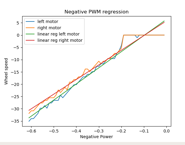
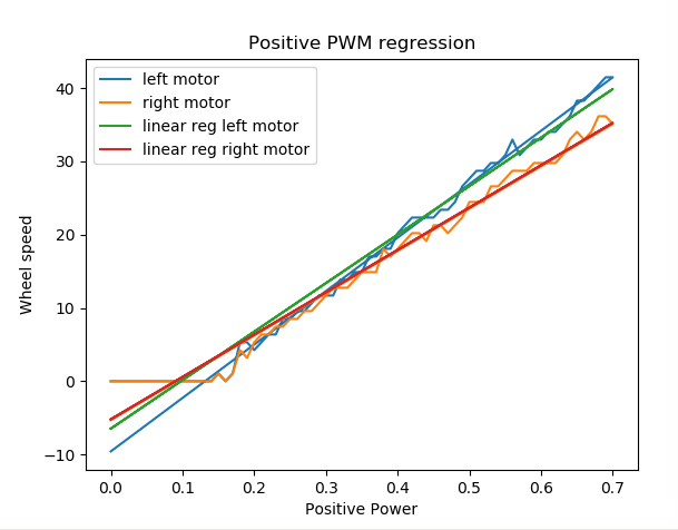
One of the problem first we encountered while working on this project, was the fact that the motors did not have the same power and response: in other words for the same pwm signal in input, the motors would not drive the wheels at the same speed.
Benchmarking motors and infering "acceleration profiles" was the first step toward more accurate control, especially when driving in a straight line.
We had the motor run through different PWM values (both negative and positive) and measured the resulting speeds. We then performed simple linear regressions (using Scikit-learn) to get intermediate transform functions to be applied to the input signals in order to get more equal outputs:
Our Differential Drive kinematics library
This library contains the functions used by the robot to drive, localize itself and execute the drawing.
Differential Drive control
Original idea
Our first idea was to implement a PID controller for the angle, in order to have a smooth trajectory, instead of the start and stop strategy we used in the end. Since the dynamics of a differential drive (the dynamics that are used for our robot) are not linear and the linearization is not controllable, we decided to fix the linear speed of the robot, and only control its angle using a PID controller.
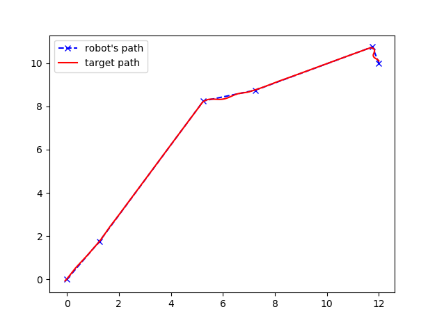
To test the correctness of our equations,We first did some path following simulations of the PID controller in python. And then we tried to implement this for the real robot, in order to have smooth drawings.
The following function was used to get the angular speed based on the displacement of the robot to the target angle.
DifferentialDrive.cpp
float DifferentialDriveKinematics::controlAngle(float angle, float target_angle) {
    float error = target_angle - angle;

    if (isItFirstExecControlAngle) {
        isItFirstExecControlAngle = false;
        previous_error = error;
    }

    float angular_speed = Kp*error + Ki*steady_error + Kd*(error-previous_error) / Ts;

    // float angular_speed = Kp*error + Ki*steady_error

    previous_error = error;
    steady_error += error*Ts;

    return angular_speed;
}
Unfortunately, the results in real life were not as good as those in simulations:
- First the motors did not have the same power (a problem we solved after trying the PID controller).
- Other factors like a faulty wheel alignment also did not help the performance of the PID controller and made it harder to gauge the performance of the system.
This is why we decided to try a simpler strategy, and have the robot first turn toward the target, and then drive to the target: we called this strategy start and stop.
Current Design
In this start/stop approach, the robots turns toward the next node it wants to go to, then it moves in a straight-line towards it, and stops once it has reached(within acceptable margin) or misses the target. This algorithm repeats until there are no more points in the path.
States management was originally done using an enum based state machine and a switch-case inside a tick() loop, however for readability we switched toward independents functions.
The pen is operated at the beginning of each segment, based on the actuation command issued during drawing creation.
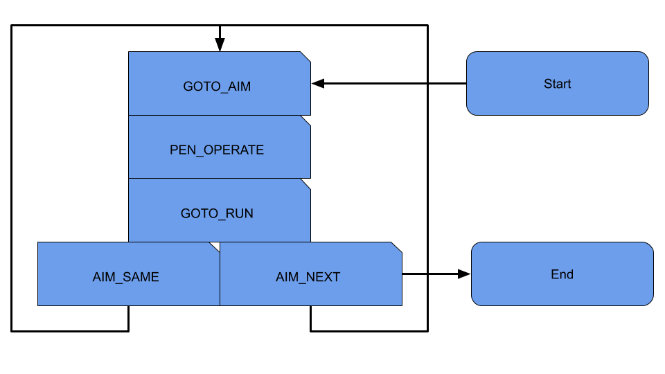 Each stages are interleaved with a complete stop of the robot, it allows for an easier assessment of accumulated drift.
Additionnally we experimeted with getting the Pen-off the surface during the rotation phase and driving in reverse for a short time, in order to get the robot to draw connected lines without the artefacts during rotations (see Square example in the Demo Section).
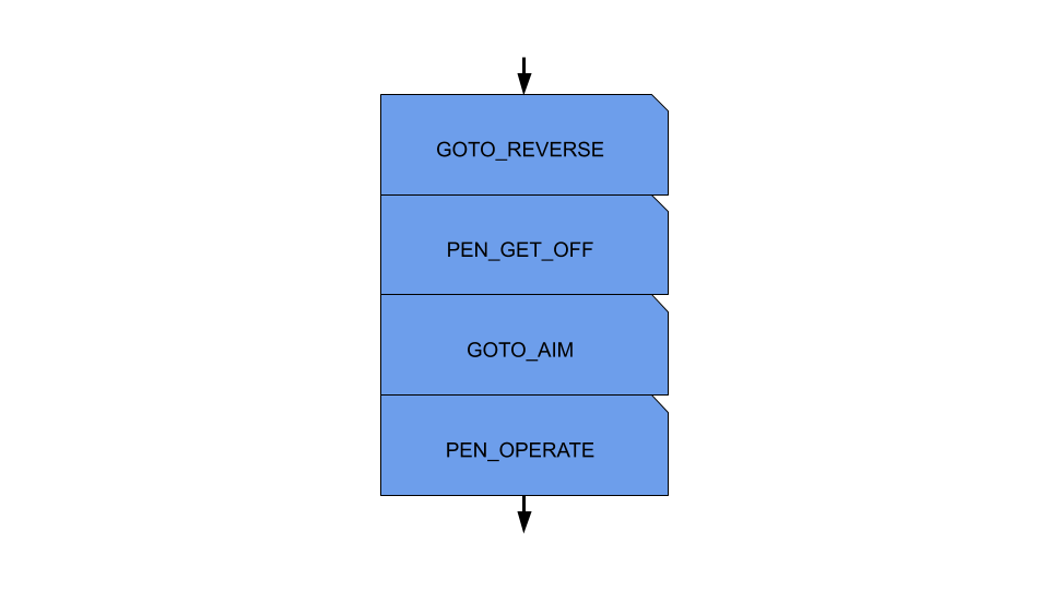
Information
This part of the code sits inside the function followPath()
Localization
Original idea
We tried to perform localization solely with encoders odometry, we use the dynamics of a differential drive in order to update the states of the robot (x, y, theta).
DifferentialDriveKinematics.cpp
void DifferentialDriveKinematics::updateStates(float speed_left, float speed_right) {
    _x = _x + Ts*(R / 2.0)*((speed_left + speed_right) / R)*cos(_theta);
    _y = _y + Ts*(R / 2.0)*((speed_left + speed_right) / R)*sin(_theta);

    float pi = PI;
    float temp = _theta + Ts*(R / L)*((speed_right - speed_left) / R);
    _theta = fmod(temp + pi, 2*pi) - pi;
}
This Method has has proven to be effective at assessing the driving distance on straight lines, however the theta was off by a large margin, this is why we has to introduce IMU readings to correct this measure.
Attempt at IMU Correction
Already having experience with kalman filters, we tried to get the best of both worlds by performing sensors fusion of both the encoders odometry and the IMU readings, by chaining them one after the other :
The code looked like this:
Kalman
       // PREDICT
        float previous_states[3];
        previous_states[0] = _x;
        previous_states[1] = _y;
        previous_states[2] = _theta;

        float predicted_states[3];

        kalmanPredict(command_speed_left, command_speed_right, predicted_states);

        // UPDATE WHEELS
        float observed_states[3];
        observed_states[0] = 0.0;
        observed_states[1] = 0.0;
        observed_states[2] = 0.0;

        dynamicsWheels(real_speed_left, real_speed_right, previous_states, observed_states);
         kalmanUpdate(observed_states, predicted_states, fp, false);

        // UPDATE IMU
        predicted_states[0] = _x;
        predicted_states[1] = _y;
        predicted_states[2] = _theta;

        float linear_speed     = getLinearSpeedFromIMU();
        float angular_speed = getAngularSpeedFromIMU();

        dynamicsIMU(linear_speed, angular_speed, previous_states, observed_states);

        kalmanUpdate(observed_states, predicted_states, fp,true );
Computations as done using the Eigen library (http://eigen.tuxfamily.org/), using an MBed port available at: https://os.mbed.com/users/ykuroda/code/Eigen/.
If you are not familliar with Kalman Filters, we higly recommend to understand the following computations the paper "An Introduction to Kalman Filters - Greg Welch and Gary Bishop". PDF: https://www.cs.unc.edu/~welch/media/pdf/kalman_intro.pdf
Kalman Predict
void DifferentialDriveKinematics::kalmanPredict(float speed_left, float speed_right, float predicted_states[3], bool imu = false) {

    float previous_states[3];
    previous_states[0] = _x;
    previous_states[1] = _y;
    previous_states[2] = _theta;

    dynamicsWheels(speed_left, speed_right, previous_states, predicted_states);

    Eigen::Matrix3f& Rk = Rk_odo;
    if(imu){
        Rk = Rk_imu;
    }

    Fk << 1, 0, -((speed_left + speed_right)/2)*sin(previous_states[2]),
          0, 1, ((speed_left + speed_right)/2)*cos(previous_states[2]),
          0, 0, 1;

    Pk = Fk*Pk*Fk.transpose() + Qk;

}
Kalman Update
void DifferentialDriveKinematics::kalmanUpdate(float observed_states[3], float predicted_states[3], FILE* fp, bool imu = false) {

    float error_x = observed_states[0] - predicted_states[0];
    float error_y = observed_states[1] - predicted_states[1];
    float error_theta = observed_states[2] - predicted_states[2];


    Eigen::Matrix3f& Rk = Rk_odo;
    if(imu){
        Rk = Rk_imu;
    }

    Eigen::Vector3f yk;
    yk << error_x, error_y, error_theta;

    Eigen::Matrix3f Sk = Hk*Pk*Hk.transpose() + Rk;

    Eigen::Matrix3f Kk = Pk*Hk.transpose()*Sk.inverse();

    Eigen::Vector3f temp = Kk*yk;

    _x = predicted_states[0] + temp(0);
    _y = predicted_states[1] + temp(1);
    _theta = predicted_states[2] + temp(2);

    Eigen::Matrix3f eye;
    eye << 1, 0, 0,
           0, 1, 0,
           0, 0, 1;

    Pk = (eye - Kk*Hk)*Pk;

}
Current Design
We observed only after implementing this that:
- Wheels odometry was very bad at determining the robot's angle, the IMU did a better job (but not a perfect one)
- Accelerometer readings were still biased after calibration and too jittery for our accuracy needs.
We decided to use only the Gyroscope readings for the angle and dropped the use of Accelerometer. Therefore those sensors did not need any cooperation anymore and we dropped the Kalman Filter altogether.
In this current state, the robot still has a major drift problem with regards to rotations, we suppose beyond the accuracy of the gyroscope.
Drawing Software
WIth the overconfidence that we could make a software in which we could free-hand draw a design and convert it to curves/subsample it to get paths made of points, we first headed toward some heavy duty GUI frameworks that offered interactive drawing capabilities. We experimented quite some time with WxWidgets (https://www.wxwidgets.org/), a convieniently crossplatform library that already offered most of the features we were looking for. However, the learning curve was just too steep and quickly reconsidered the need for that much sophistication in the drawing software given the capabilities of our robot.
In the end, we developed a fairly simple Python application based on Tkinter library. It allows the management (create/save/load) of drawing projects, where one can place a set of nodesin a fixed-size drawing-area in order to describe a drawing path. Each node can be set to be "drawing" (green) or not (red), enabling the user to make a drawing made of discontinued segments.
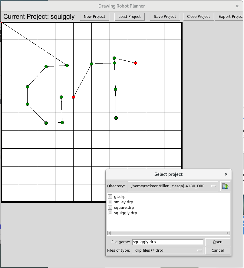
The software can then export the drawing to a csv-like format, understandable by the robot.
Here is a presentation of the software in video:
Uploading the Drawing to the robot
We originally wanted to perform the upload by bluetooth, however we never got to make the Bluefruit chip to work.
Thefore we have to manually supply it using the SD card reader on the robot. The file we supply to the robot is a .csv file, and in order to extract the data from this file, we created the following function that the robot uses in order to know where to go and when to use the pencil.
Information
This part of the code is available in the function path_parser(Path path, FILE* fp) of main.cpp
Debugging framework
Logging system
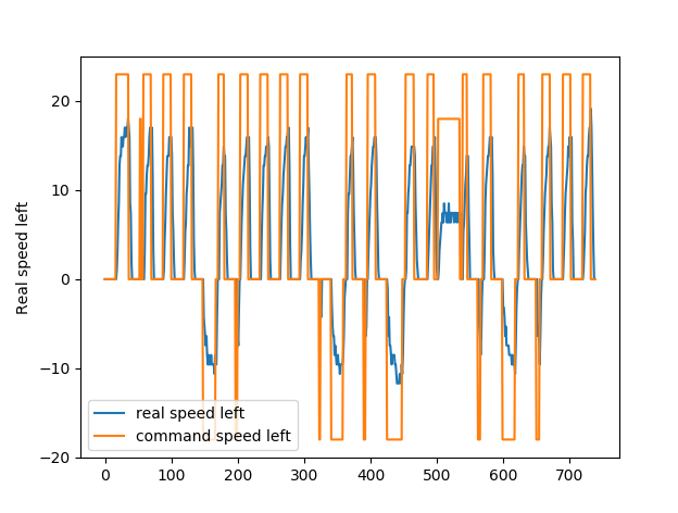
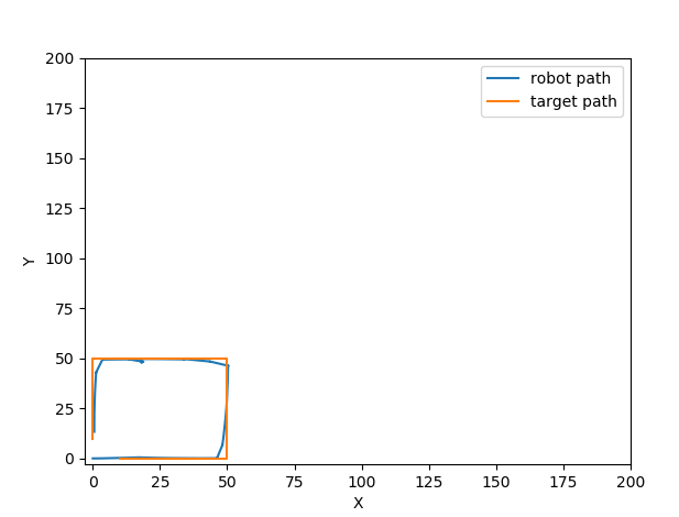
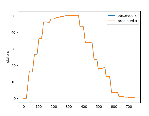
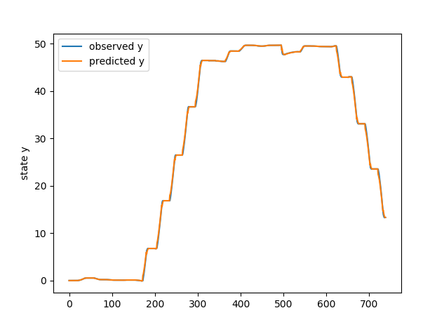
To debug the robot's behavior and kinematics, we developped a set of Python scripts that allowed us to process logs produced at runtime and written to the SD Card.
The following log is one from our best runs at a square path, before integration of the servo/Pen and without the weight of the battery, those were optimal conditions:
Demo
In its current state, the robot can only reproduce very basic recognisable shapes due to its inaccuracies with regards to angle assessment.
We will illustrate the different features of the robot and its accuracy in the following videos.
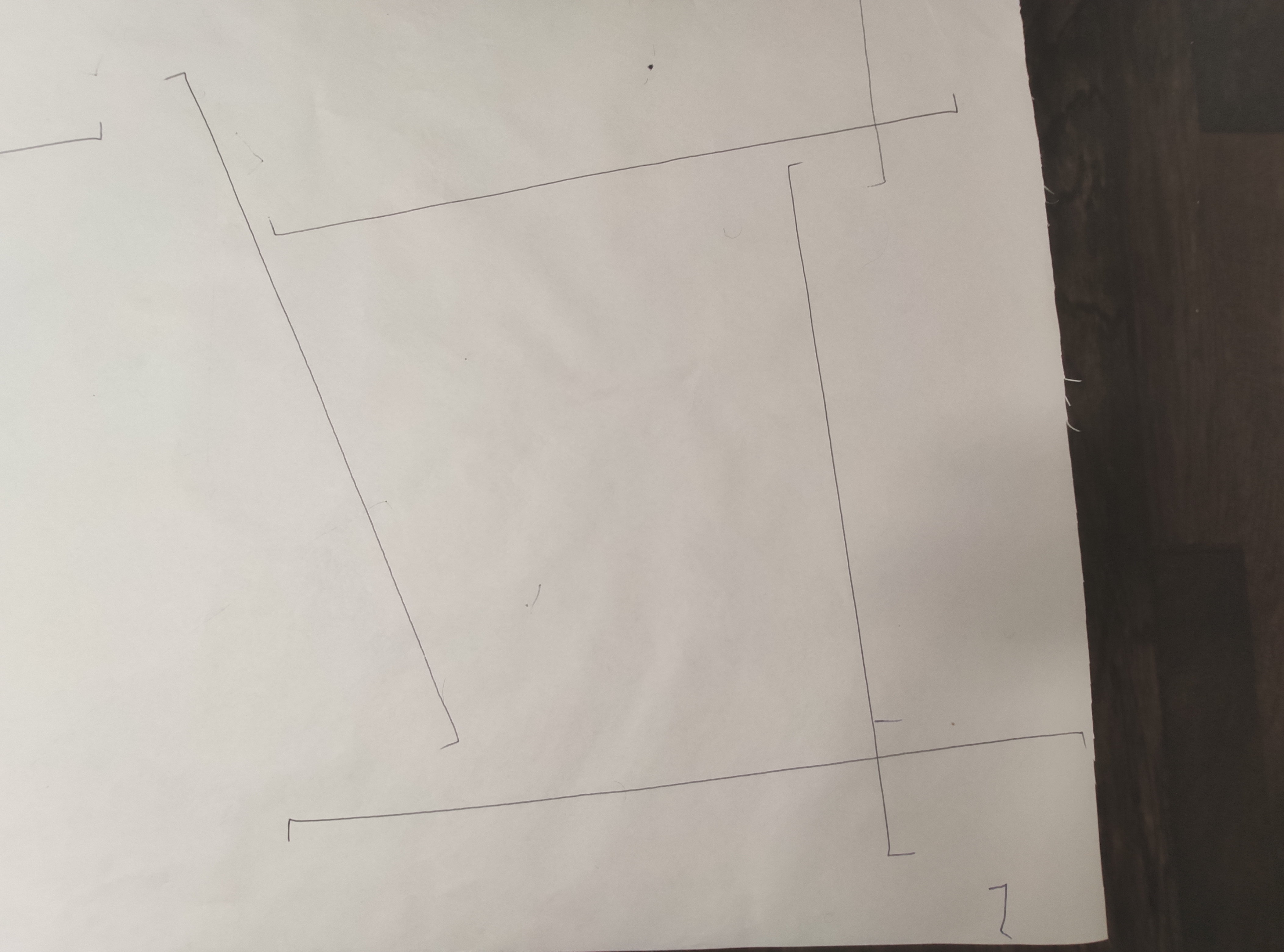
We apologise for the fact that the sheet of papers are cluttered, but we ran out of paper after experimenting quite a lot of times.
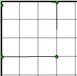
Square Example
The square example, gives a good sense of the achieved accuracy and illustrates our "Reverse and lift the pen" Method for connected drawings:
Octogon Example
Trying an more complex example like an octogon, quicly highlighted the weakness of the system : inaccurate angle measures.
In this Octogon example, we decided to keep the Pen down all the time to get a better understanding of the trajectory.
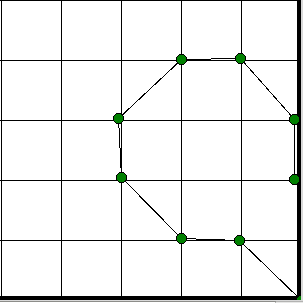
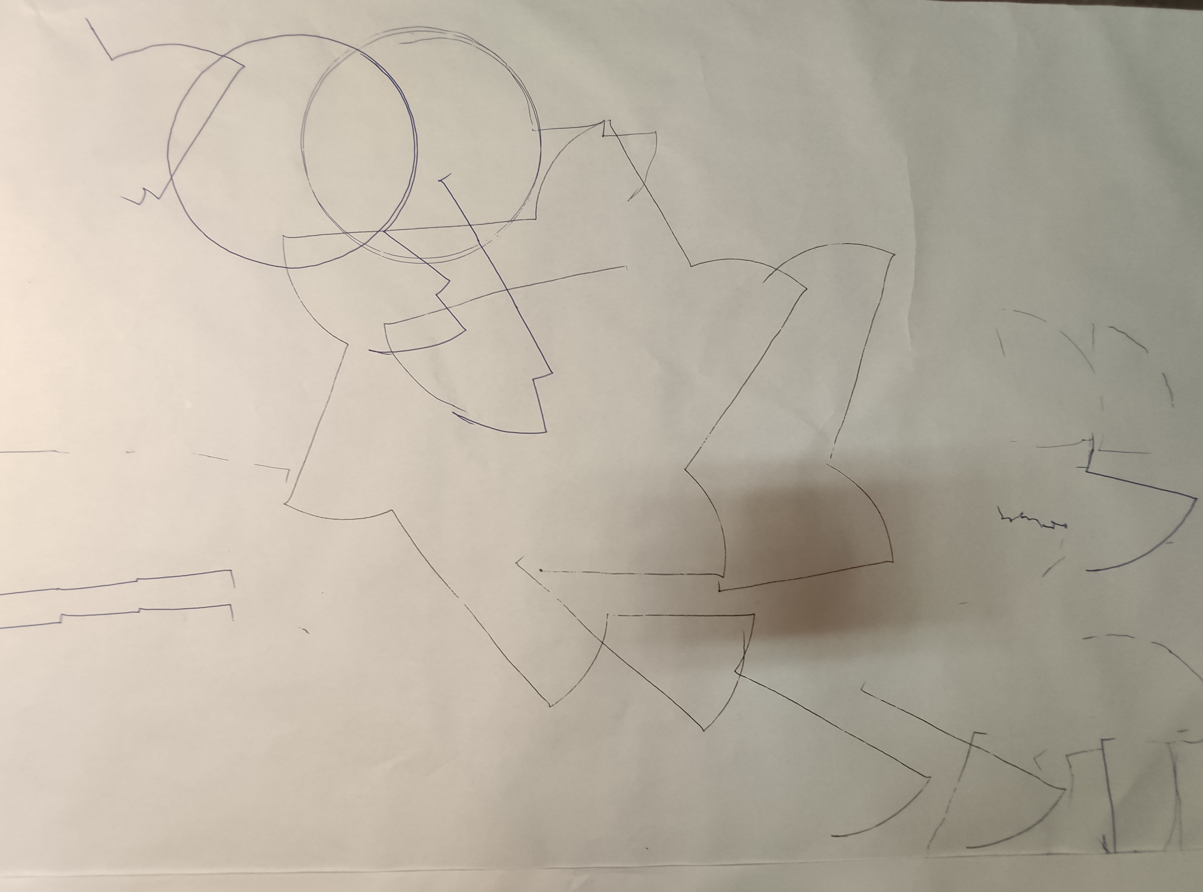
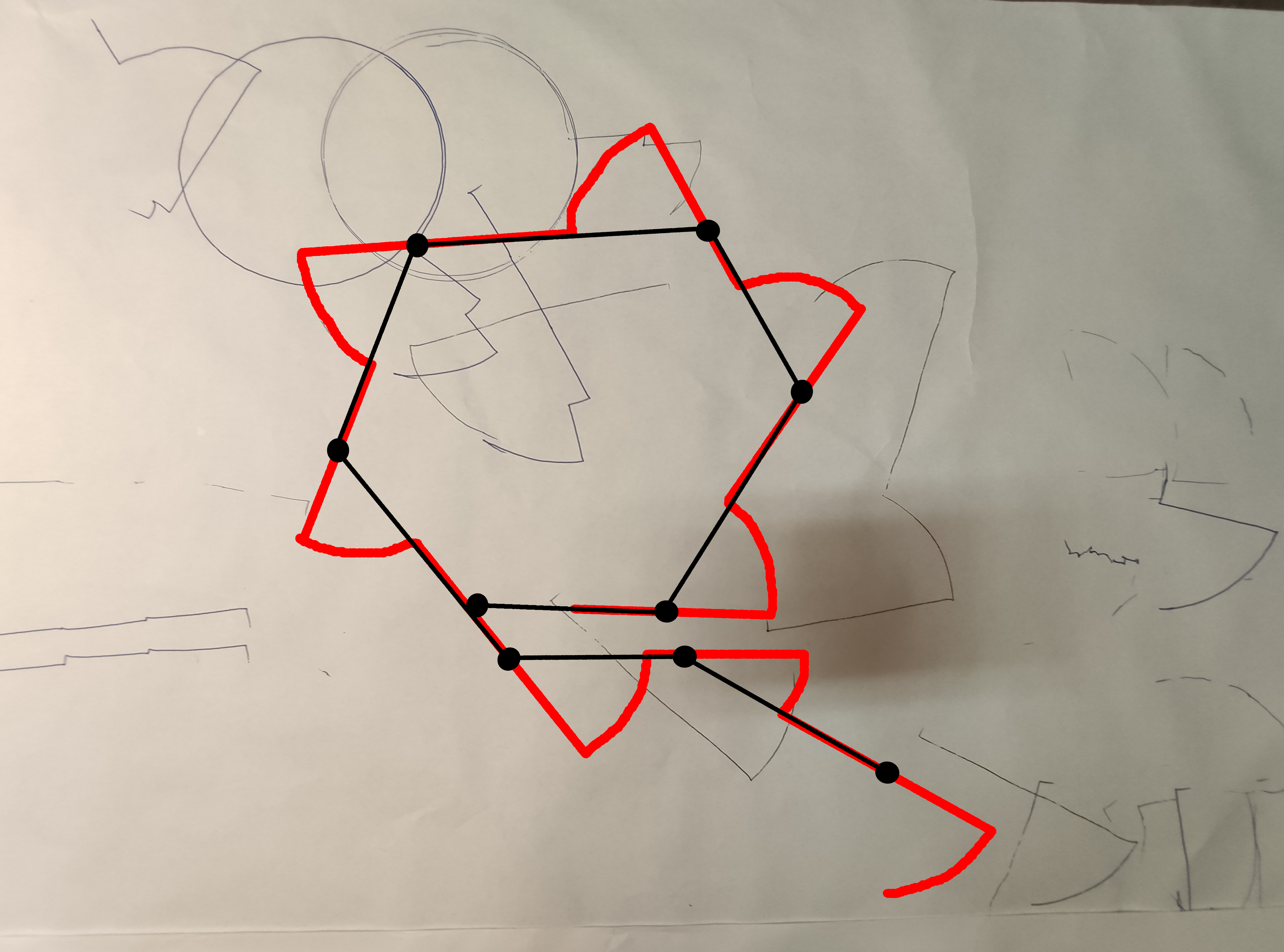
We can see that the resulting path mostly overshoot rotations and endedup drawing more an hexagon instead of an octogon, overlapping the last segment.
We used the same example to demonstrate the features of our system, first the ability to lift the Pen during rotation if wanted:
Secondly, the ability to draw using disconnected componnents, here we decided to draw only one side alternatively:
Improvements
Aside from the inability to make the bluetooth chip work and that our drawing software could use quite some refinning, we will focus our discussion on improving accuracy:
We were not able to implement a satisfyingly enough control algorithm for this system, we explored both wheels odometry and IMU to solve the localization problem with relative success. We have a few concerns with how we integrated the encoders/IMU updates, especially with the frequency and the async nature their update; or maybe the kalman filter should have been used at the sensors level and not at the dynamics level.
Overall we feel that there is little more we could have done to fight drift, at least with what we had and our knowledge. We now realise that the task of drawing something accurately without a proper SLAM system is tedious and maybe we should have looked onto that a bit earlier.
Additionally, we felt a bit helpless against the mechanical problems we encountered: - Uneven floor, either a somewhat curved wooden floor or a rough concrete of the garage - Plastic Wheels sliding on the paper - Tying the Pen at the right distance to create less friction - Dealing with the rather brute-force "noisy" actuation of the Pen, jerking the robot
Heres an example of the robot slidding on paper, having catastrophic impact on the localization accuracy :
Conclusion
After countless hours debugging code, inspecting logs, fine-tuning parameters, replacing the sharpie and unrolling paper, we achieved the basic features of our project. We may not have reached an outstanding level performance but we tried to get the most out of what we had and what we knew.
On a project management point of view, despite being not in the same area and only one of us had access to the robot, we managed to split the work quite nicely, between the MBED code, the software-sdcard pipeline or analysing control logs.
Please log in to post comments.
